MATLAB lessons N.2
All MATLAB file for the lesson in a unique archive lesson2.zip
Exercise on MATLAB ode solver
Example of ODE solver of MATLAB
File ode1.m
:open:
 1function Y = ode1(odefun,tspan,y0,varargin)
 2%ODE1  Solve differential equations with a non-adaptive method of order 1.
 3%   Y = ODE1(ODEFUN,TSPAN,Y0) with TSPAN = [T1, T2, T3, ... TN] integrates
 4%   the system of differential equations y' = f(t,y) by stepping from T0 to
 5%   T1 to TN. Function ODEFUN(T,Y) must return f(t,y) in a column vector.
 6%   The vector Y0 is the initial conditions at T0. Each row in the solution
 7%   array Y corresponds to a time specified in TSPAN.
 8%
 9%   Y = ODE1(ODEFUN,TSPAN,Y0,P1,P2...) passes the additional parameters
10%   P1,P2... to the derivative function as ODEFUN(T,Y,P1,P2...).
11%
12%   This is a non-adaptive solver. The step sequence is determined by TSPAN.
13%   The solver implements the forward Euler method of order 1.
14%
15%   Example
16%         tspan = 0:0.1:20;
17%         y = ode1(@vdp1,tspan,[2 0]);
18%         plot(tspan,y(:,1));
19%     solves the system y' = vdp1(t,y) with a constant step size of 0.1,
20%     and plots the first component of the solution.
21%
22
23if ~isnumeric(tspan)
24  error('TSPAN should be a vector of integration steps.');
25end
26
27if ~isnumeric(y0)
28  error('Y0 should be a vector of initial conditions.');
29end
30
31h = diff(tspan);
32if any(sign(h(1))*h <= 0)
33  error('Entries of TSPAN are not in order.')
34end
35
36try
37  f0 = feval(odefun,tspan(1),y0,varargin{:});
38catch
39  msg = ['Unable to evaluate the ODEFUN at t0,y0. ',lasterr];
40  error(msg);
41end
42
43y0 = y0(:);   % Make a column vector.
44if ~isequal(size(y0),size(f0))
45  error('Inconsistent sizes of Y0 and f(t0,y0).');
46end
47
48neq = length(y0);
49N = length(tspan);
50Y = zeros(neq,N);
51
52Y(:,1) = y0;
53for i = 1:N-1
54  Y(:,i+1) = Y(:,i) + h(i)*feval(odefun,tspan(i),Y(:,i),varargin{:});
55end
56Y = Y.';
output of the command:
Changing tolerance parameters:
File test2.m
:open:
1%
2% Example of ODE solver of MATLAB
3%
4
5% set some option for the ODE numerical solver
6options = odeset('RelTol',1e-7,'AbsTol',[1e-7 1e-7 1e-7]);
7
8% se initial condition for the problem
9Y0 = [ -7.5 -3.6 30 ] ;
10
11% Set a vector specifying the interval of integration, [t0,tf].
12% The solver imposes the initial conditions at TSPAN(1),
13% and integrates from TSPAN(1) to TSPAN(end).
14% To obtain solutions at specific times (all increasing or all decreasing),
15% use TSPAN = [t0,t1,...,tf].
16TSPAN = [ 0:0.01:10 ] ;
17
18% load the "pointer" of the function to FUN
19FUN = @lorenz ;
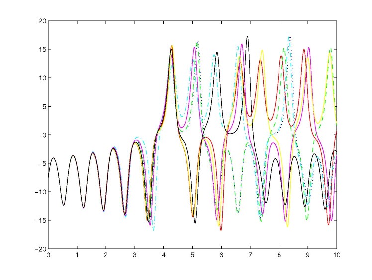
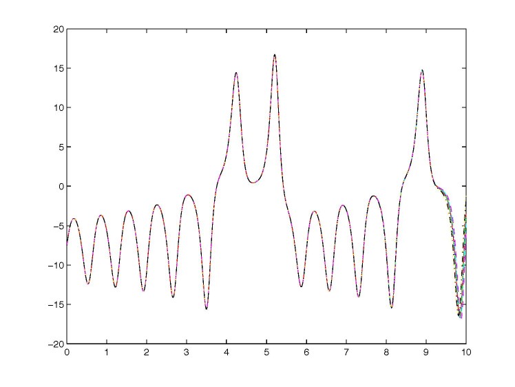
20
21% Runge-Kutta embedded of order 2 and 3 by Bogaci and Shampine
22[T1,Y1] = ode23 ( FUN, TSPAN, Y0, options ) ;
23
24% Runge-Kutta embedded of order 4 and 5 by Dormand and Prince (first choice scheme)
25[T2,Y2] = ode45 ( FUN, TSPAN, Y0, options ) ;
26
27% Adams-bashforth-Moulton PECE
28[T3,Y3] = ode113 ( FUN, TSPAN, Y0, options ) ;
29
30% Numerical Differentiation Formula, similar to Backward Differetiation Formula
31% by Gear. Useful for stiff problem.
32[T4,Y4] = ode15s ( FUN, TSPAN, Y0, options ) ;
33
34% Rosenbrock of order 2. For stiff problem.
35[T5,Y5] = ode23s ( FUN, TSPAN, Y0, options ) ;
36
37% Trapeziodal rule for moderately stiff problem
38[T6,Y6] = ode23t ( FUN, TSPAN, Y0, options ) ;
39
40% TR-BDF2 an implit Runge-Kutta where the first stage is the
41% trapezoidal rule and teh second stage is a BDF formula of order 2
42[T7,Y7] = ode23tb ( FUN, TSPAN, Y0, options ) ;
43
44%
45% plot the functions approximated by various solver
46%
47plot( T1, Y1(:,1), 'r-', ...
48 T2, Y2(:,1), 'g--', ...
49 T3, Y3(:,1), 'b:', ...
50 T4, Y4(:,1), 'c-.', ...
51 T5, Y5(:,1), 'm--', ...
52 T6, Y6(:,1), 'y:', ...
53 T7, Y7(:,1), 'k-.' )
this is the output of the command
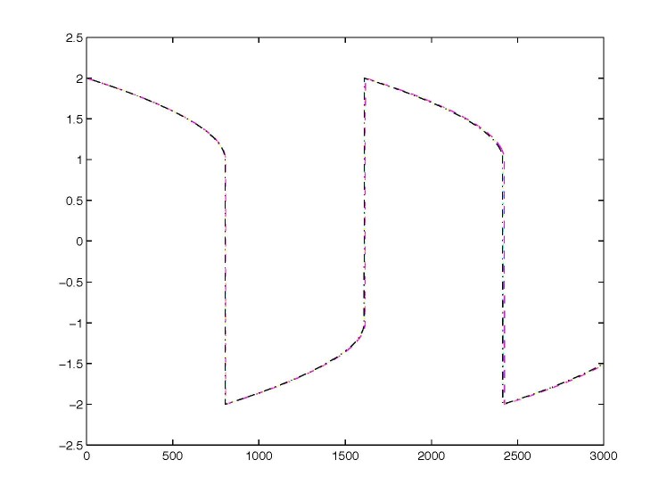
File test3.m
:open:
1%
2% Check Van Der Pol equation
3% this is a stiff test
4%
5
6% set some option for the ODE numerical solver
7options = odeset('RelTol',1e-4) ; %,'AbsTol',[1e-7 1e-7 1e-7]);
8
9% se initial condition for the problem
10Y0 = [ 2 0 ] ;
11
12% Set a vector specifying the interval of integration, [t0,tf].
13% The solver imposes the initial conditions at TSPAN(1),
14% and integrates from TSPAN(1) to TSPAN(end).
15% To obtain solutions at specific times (all increasing or all decreasing),
16% use TSPAN = [t0,t1,...,tf].
17TSPAN = [ 0:1:3000 ] ;
18
19% load the "pointer" of the function to FUN
20FUN = @vanderpol ;
21
22% This is a stiff problem, the first three solver do not work!
23%[T1,Y1] = ode23 ( FUN, TSPAN, Y0 ) ;
24%[T2,Y2] = ode45 ( FUN, TSPAN, Y0 ) ;
25%[T3,Y3] = ode113 ( FUN, TSPAN, Y0 ) ;
26
27% those solvers can solve a stiff problem
28[T4,Y4] = ode15s ( FUN, TSPAN, Y0 ) ;
29[T5,Y5] = ode23s ( FUN, TSPAN, Y0 ) ;
30[T6,Y6] = ode23t ( FUN, TSPAN, Y0 ) ;
31[T7,Y7] = ode23tb ( FUN, TSPAN, Y0 ) ;
32
33%
34% plot the functions approximated by various solver
35%
36% first component
37plot( T4, Y4(:,1), 'c-.', ...
38 T5, Y5(:,1), 'm--', ...
39 T6, Y6(:,1), 'y:', ...
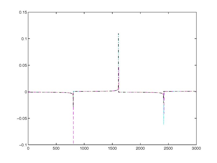
40 T7, Y7(:,1), 'k-.' )
41
42% create a new window to plot
43figure()
44
45% second component
46plot( T4, Y4(:,2), 'c-.', ...
47 T5, Y5(:,2), 'm--', ...
48 T6, Y6(:,2), 'y:', ...
49 T7, Y7(:,2), 'k-.' )
this is the output of the command
and this
Numerical ODE solver with constants step size
This routine are taken from mathworks
First order explicit Euler:
File ode1.m
:open:
 1function Y = ode1(odefun,tspan,y0,varargin)
 2%ODE1  Solve differential equations with a non-adaptive method of order 1.
 3%   Y = ODE1(ODEFUN,TSPAN,Y0) with TSPAN = [T1, T2, T3, ... TN] integrates
 4%   the system of differential equations y' = f(t,y) by stepping from T0 to
 5%   T1 to TN. Function ODEFUN(T,Y) must return f(t,y) in a column vector.
 6%   The vector Y0 is the initial conditions at T0. Each row in the solution
 7%   array Y corresponds to a time specified in TSPAN.
 8%
 9%   Y = ODE1(ODEFUN,TSPAN,Y0,P1,P2...) passes the additional parameters
10%   P1,P2... to the derivative function as ODEFUN(T,Y,P1,P2...).
11%
12%   This is a non-adaptive solver. The step sequence is determined by TSPAN.
13%   The solver implements the forward Euler method of order 1.
14%
15%   Example
16%         tspan = 0:0.1:20;
17%         y = ode1(@vdp1,tspan,[2 0]);
18%         plot(tspan,y(:,1));
19%     solves the system y' = vdp1(t,y) with a constant step size of 0.1,
20%     and plots the first component of the solution.
21%
22
23if ~isnumeric(tspan)
24  error('TSPAN should be a vector of integration steps.');
25end
26
27if ~isnumeric(y0)
28  error('Y0 should be a vector of initial conditions.');
29end
30
31h = diff(tspan);
32if any(sign(h(1))*h <= 0)
33  error('Entries of TSPAN are not in order.')
34end
35
36try
37  f0 = feval(odefun,tspan(1),y0,varargin{:});
38catch
39  msg = ['Unable to evaluate the ODEFUN at t0,y0. ',lasterr];
40  error(msg);
41end
42
43y0 = y0(:);   % Make a column vector.
44if ~isequal(size(y0),size(f0))
45  error('Inconsistent sizes of Y0 and f(t0,y0).');
46end
47
48neq = length(y0);
49N = length(tspan);
50Y = zeros(neq,N);
51
52Y(:,1) = y0;
53for i = 1:N-1
54  Y(:,i+1) = Y(:,i) + h(i)*feval(odefun,tspan(i),Y(:,i),varargin{:});
55end
56Y = Y.';
Second order explicit Runge Kutta:
File ode2.m
:open:
 1function Y = ode2(odefun,tspan,y0,varargin)
 2%ODE2  Solve differential equations with a non-adaptive method of order 2.
 3%   Y = ODE2(ODEFUN,TSPAN,Y0) with TSPAN = [T1, T2, T3, ... TN] integrates
 4%   the system of differential equations y' = f(t,y) by stepping from T0 to
 5%   T1 to TN. Function ODEFUN(T,Y) must return f(t,y) in a column vector.
 6%   The vector Y0 is the initial conditions at T0. Each row in the solution
 7%   array Y corresponds to a time specified in TSPAN.
 8%
 9%   Y = ODE2(ODEFUN,TSPAN,Y0,P1,P2...) passes the additional parameters
10%   P1,P2... to the derivative function as ODEFUN(T,Y,P1,P2...).
11%
12%   This is a non-adaptive solver. The step sequence is determined by TSPAN
13%   but the derivative function ODEFUN is evaluated multiple times per step.
14%   The solver implements the improved Euler (Heun's) method of order 2.
15%
16%   Example
17%         tspan = 0:0.1:20;
18%         y = ode2(@vdp1,tspan,[2 0]);
19%         plot(tspan,y(:,1));
20%     solves the system y' = vdp1(t,y) with a constant step size of 0.1,
21%     and plots the first component of the solution.
22%
23
24if ~isnumeric(tspan)
25  error('TSPAN should be a vector of integration steps.');
26end
27
28if ~isnumeric(y0)
29  error('Y0 should be a vector of initial conditions.');
30end
31
32h = diff(tspan);
33if any(sign(h(1))*h <= 0)
34  error('Entries of TSPAN are not in order.')
35end
36
37try
38  f0 = feval(odefun,tspan(1),y0,varargin{:});
39catch
40  msg = ['Unable to evaluate the ODEFUN at t0,y0. ',lasterr];
41  error(msg);
42end
43
44y0 = y0(:);   % Make a column vector.
45if ~isequal(size(y0),size(f0))
46  error('Inconsistent sizes of Y0 and f(t0,y0).');
47end
48
49neq = length(y0);
50N = length(tspan);
51Y = zeros(neq,N);
52F = zeros(neq,2);
53
54Y(:,1) = y0;
55for i = 2:N
56  ti = tspan(i-1);
57  hi = h(i-1);
58  yi = Y(:,i-1);
59  F(:,1) = feval(odefun,ti,yi,varargin{:});
60  F(:,2) = feval(odefun,ti+hi,yi+hi*F(:,1),varargin{:});
61  Y(:,i) = yi + (hi/2)*(F(:,1) + F(:,2));
62end
63Y = Y.';
3rd order explicit Runge Kutta:
File ode3.m
:open:
 1function Y = ode3(odefun,tspan,y0,varargin)
 2%ODE3  Solve differential equations with a non-adaptive method of order 3.
 3%   Y = ODE3(ODEFUN,TSPAN,Y0) with TSPAN = [T1, T2, T3, ... TN] integrates
 4%   the system of differential equations y' = f(t,y) by stepping from T0 to
 5%   T1 to TN. Function ODEFUN(T,Y) must return f(t,y) in a column vector.
 6%   The vector Y0 is the initial conditions at T0. Each row in the solution
 7%   array Y corresponds to a time specified in TSPAN.
 8%
 9%   Y = ODE3(ODEFUN,TSPAN,Y0,P1,P2...) passes the additional parameters
10%   P1,P2... to the derivative function as ODEFUN(T,Y,P1,P2...).
11%
12%   This is a non-adaptive solver. The step sequence is determined by TSPAN
13%   but the derivative function ODEFUN is evaluated multiple times per step.
14%   The solver implements the Bogacki-Shampine Runge-Kutta method of order 3.
15%
16%   Example
17%         tspan = 0:0.1:20;
18%         y = ode3(@vdp1,tspan,[2 0]);
19%         plot(tspan,y(:,1));
20%     solves the system y' = vdp1(t,y) with a constant step size of 0.1,
21%     and plots the first component of the solution.
22%
23
24if ~isnumeric(tspan)
25  error('TSPAN should be a vector of integration steps.');
26end
27
28if ~isnumeric(y0)
29  error('Y0 should be a vector of initial conditions.');
30end
31
32h = diff(tspan);
33if any(sign(h(1))*h <= 0)
34  error('Entries of TSPAN are not in order.')
35end
36
37try
38  f0 = feval(odefun,tspan(1),y0,varargin{:});
39catch
40  msg = ['Unable to evaluate the ODEFUN at t0,y0. ',lasterr];
41  error(msg);
42end
43
44y0 = y0(:);   % Make a column vector.
45if ~isequal(size(y0),size(f0))
46  error('Inconsistent sizes of Y0 and f(t0,y0).');
47end
48
49neq = length(y0);
50N = length(tspan);
51Y = zeros(neq,N);
52F = zeros(neq,3);
53
54Y(:,1) = y0;
55for i = 2:N
56  ti = tspan(i-1);
57  hi = h(i-1);
58  yi = Y(:,i-1);
59  F(:,1) = feval(odefun,ti,yi,varargin{:});
60  F(:,2) = feval(odefun,ti+0.5*hi,yi+0.5*hi*F(:,1),varargin{:});
61  F(:,3) = feval(odefun,ti+0.75*hi,yi+0.75*hi*F(:,2),varargin{:});
62  Y(:,i) = yi + (hi/9)*(2*F(:,1) + 3*F(:,2) + 4*F(:,3));
63end
64Y = Y.';
4th order explicit Runge Kutta:
File ode4.m
:open:
 1function Y = ode4(odefun,tspan,y0,varargin)
 2%ODE4  Solve differential equations with a non-adaptive method of order 4.
 3%   Y = ODE4(ODEFUN,TSPAN,Y0) with TSPAN = [T1, T2, T3, ... TN] integrates
 4%   the system of differential equations y' = f(t,y) by stepping from T0 to
 5%   T1 to TN. Function ODEFUN(T,Y) must return f(t,y) in a column vector.
 6%   The vector Y0 is the initial conditions at T0. Each row in the solution
 7%   array Y corresponds to a time specified in TSPAN.
 8%
 9%   Y = ODE4(ODEFUN,TSPAN,Y0,P1,P2...) passes the additional parameters
10%   P1,P2... to the derivative function as ODEFUN(T,Y,P1,P2...).
11%
12%   This is a non-adaptive solver. The step sequence is determined by TSPAN
13%   but the derivative function ODEFUN is evaluated multiple times per step.
14%   The solver implements the classical Runge-Kutta method of order 4.
15%
16%   Example
17%         tspan = 0:0.1:20;
18%         y = ode4(@vdp1,tspan,[2 0]);
19%         plot(tspan,y(:,1));
20%     solves the system y' = vdp1(t,y) with a constant step size of 0.1,
21%     and plots the first component of the solution.
22%
23
24if ~isnumeric(tspan)
25  error('TSPAN should be a vector of integration steps.');
26end
27
28if ~isnumeric(y0)
29  error('Y0 should be a vector of initial conditions.');
30end
31
32h = diff(tspan);
33if any(sign(h(1))*h <= 0)
34  error('Entries of TSPAN are not in order.')
35end
36
37try
38  f0 = feval(odefun,tspan(1),y0,varargin{:});
39catch
40  msg = ['Unable to evaluate the ODEFUN at t0,y0. ',lasterr];
41  error(msg);
42end
43
44y0 = y0(:);   % Make a column vector.
45if ~isequal(size(y0),size(f0))
46  error('Inconsistent sizes of Y0 and f(t0,y0).');
47end
48
49neq = length(y0);
50N = length(tspan);
51Y = zeros(neq,N);
52F = zeros(neq,4);
53
54Y(:,1) = y0;
55for i = 2:N
56  ti = tspan(i-1);
57  hi = h(i-1);
58  yi = Y(:,i-1);
59  F(:,1) = feval(odefun,ti,yi,varargin{:});
60  F(:,2) = feval(odefun,ti+0.5*hi,yi+0.5*hi*F(:,1),varargin{:});
61  F(:,3) = feval(odefun,ti+0.5*hi,yi+0.5*hi*F(:,2),varargin{:});
62  F(:,4) = feval(odefun,tspan(i),yi+hi*F(:,3),varargin{:});
63  Y(:,i) = yi + (hi/6)*(F(:,1) + 2*F(:,2) + 2*F(:,3) + F(:,4));
64end
65Y = Y.';
5th order explicit Runge Kutta:
File ode5.m
:open:
 1function Y = ode5(odefun,tspan,y0,varargin)
 2%ODE5  Solve differential equations with a non-adaptive method of order 5.
 3%   Y = ODE5(ODEFUN,TSPAN,Y0) with TSPAN = [T1, T2, T3, ... TN] integrates
 4%   the system of differential equations y' = f(t,y) by stepping from T0 to
 5%   T1 to TN. Function ODEFUN(T,Y) must return f(t,y) in a column vector.
 6%   The vector Y0 is the initial conditions at T0. Each row in the solution
 7%   array Y corresponds to a time specified in TSPAN.
 8%
 9%   Y = ODE5(ODEFUN,TSPAN,Y0,P1,P2...) passes the additional parameters
10%   P1,P2... to the derivative function as ODEFUN(T,Y,P1,P2...).
11%
12%   This is a non-adaptive solver. The step sequence is determined by TSPAN
13%   but the derivative function ODEFUN is evaluated multiple times per step.
14%   The solver implements the Dormand-Prince method of order 5 in a general
15%   framework of explicit Runge-Kutta methods.
16%
17%   Example
18%         tspan = 0:0.1:20;
19%         y = ode5(@vdp1,tspan,[2 0]);
20%         plot(tspan,y(:,1));
21%     solves the system y' = vdp1(t,y) with a constant step size of 0.1,
22%     and plots the first component of the solution.
23
24if ~isnumeric(tspan)
25  error('TSPAN should be a vector of integration steps.');
26end
27
28if ~isnumeric(y0)
29  error('Y0 should be a vector of initial conditions.');
30end
31
32h = diff(tspan);
33if any(sign(h(1))*h <= 0)
34  error('Entries of TSPAN are not in order.')
35end
36
37try
38  f0 = feval(odefun,tspan(1),y0,varargin{:});
39catch
40  msg = ['Unable to evaluate the ODEFUN at t0,y0. ',lasterr];
41  error(msg);
42end
43
44y0 = y0(:);   % Make a column vector.
45if ~isequal(size(y0),size(f0))
46  error('Inconsistent sizes of Y0 and f(t0,y0).');
47end
48
49neq = length(y0);
50N = length(tspan);
51Y = zeros(neq,N);
52
53% Method coefficients -- Butcher's tableau
54%
55%   C | A
56%   --+---
57%     | B
58
59C = [1/5; 3/10; 4/5; 8/9; 1];
60
61A = [ 1/5,          0,           0,            0,         0
62      3/40,         9/40,        0,            0,         0
63      44/45        -56/15,       32/9,         0,         0
64      19372/6561,  -25360/2187,  64448/6561,  -212/729,   0
65      9017/3168,   -355/33,      46732/5247,   49/176,   -5103/18656];
66
67B = [35/384, 0, 500/1113, 125/192, -2187/6784, 11/84];
68
69% More convenient storage
70A = A.';
71B = B(:);
72
73nstages = length(B);
74F = zeros(neq,nstages);
75
76Y(:,1) = y0;
77for i = 2:N
78  ti = tspan(i-1);
79  hi = h(i-1);
80  yi = Y(:,i-1);
81
82  % General explicit Runge-Kutta framework
83  F(:,1) = feval(odefun,ti,yi,varargin{:});
84  for stage = 2:nstages
85    tstage = ti + C(stage-1)*hi;
86    ystage = yi + F(:,1:stage-1)*(hi*A(1:stage-1,stage-1));
87    F(:,stage) = feval(odefun,tstage,ystage,varargin{:});
88  end
89  Y(:,i) = yi + F*(hi*B);
90
91end
92Y = Y.';
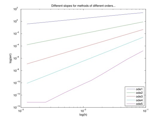
Checking the order
Graphical plot of the order:
File ode_test.m
:open:
 1function ode_test
 2%ODE_TEST  Run non-adaptive ODE solvers of different orders.
 3%   ODE_TEST compares the orders of accuracy of several explicit Runge-Kutta
 4%   methods. The non-adaptive ODE solvers are tested on a problem used in
 5%   E. Hairer, S.P. Norsett, and G. Wanner, Solving Ordinary Differential
 6%   Equations I, Nonstiff Problems, Springer-Verlag, 1987.
 7%   The errors of numerical solutions obtained with several step sizes is
 8%   plotted against the step size used. For a given solver, the slope of that
 9%   line corresponds to the order of the integration method used.
10%
11
12solvers = {'ode1','ode2','ode3','ode4','ode5'};
13Nsteps = [800 400 200 100 75 50 20 11];
14
15x0 = 0;
16y0 = [1;1;1;1];
17xend = 1;
18h = (xend-x0)./Nsteps;
19
20err = zeros(length(solvers),length(h));
21
22for i = 1:length(solvers)
23  solver = solvers{i};
24  for j = 1:length(Nsteps)
25    N = Nsteps(j);
26    x = linspace(x0,xend,N+1);
27    y = feval(solver,@f,x,y0);
28    err(i,j) = max(max(abs(y - yexact(x))));
29  end
30end
31
32figure
33loglog(h,err);
34title('Different slopes for methods of different orders...');
35xlabel('log(h)');
36ylabel('log(err)');
37legend(solvers{:},4);
38
39% -------------------------
40function yp = f(x,y)
41yp = [  2*x*y(4)*y(1)
42       10*x*y(4)*y(1)^5
43        2*x*y(4)
44       -2*x*(y(3)-1) ];
45
46% -------------------------
47function y = yexact(x)
48x2 = x(:).^2;
49y = zeros(length(x),4);
50y(:,1) = exp(sin(x2));
51y(:,2) = exp(5*sin(x2));
52y(:,3) = sin(x2)+1;
53y(:,4) = cos(x2);
Numerical estimation of the order:
File ode_check_error.m
:open:
 1function ode_check_error
 2%ODE_TEST  Run non-adaptive ODE solvers of different orders.
 3%   ODE_TEST compares the orders of accuracy of several explicit Runge-Kutta
 4%   methods. The non-adaptive ODE solvers are tested on a problem used in
 5%   E. Hairer, S.P. Norsett, and G. Wanner, Solving Ordinary Differential
 6%   Equations I, Nonstiff Problems, Springer-Verlag, 1987.
 7%   The errors of numerical solutions obtained with several step sizes is
 8%   plotted against the step size used. For a given solver, the slope of that
 9%   line corresponds to the order of the integration method used.
10%
11
12solvers = { 'ode1', 'ode2', 'ode3', 'ode4', 'ode5' };
13Nsteps  = [ 10 20 40 80 160 320 640 1280 ];
14
15x0   = 0 ;
16y0   = [1;1;1;1] ;
17xend = 1 ;
18h    = (xend-x0)./Nsteps ;
19
20err = zeros(length(solvers),length(h));
21
22for i = 1:length(solvers)
23  solver = solvers{i};
24  for j = 1:length(Nsteps)
25    N = Nsteps(j);
26    x = linspace(x0,xend,N+1);
27    y = feval(solver,@f,x,y0);
28    err(i,j) = max(max(abs(y - yexact(x))));
29  end
30end
31
32for i = 1:length(solvers)
33  disp( ' ' )
34  disp( ['estimate order for scheme = ' solvers{i}] );
35  disp( sprintf( 'Error = %-15g', err(i,1) ) ) ;
36  for j = 2:length(Nsteps)
37    order = log( err(i,j-1)/err(i,j) ) / log( h(j-1)/h(j) ) ;
38    disp( sprintf( 'Error = %-15g Order = %-15g', err(i,j), order) ) ;
39  end
40end
41
42% -------------------------
43function yp = f(x,y)
44yp = [  2*x*y(4)*y(1)
45       10*x*y(4)*y(1)^5
46        2*x*y(4)
47       -2*x*(y(3)-1) ];
48
49% -------------------------
50function y = yexact(x)
51x2 = x.^2;
52y  = zeros(length(x),4);
53y(:,1) = exp(sin(x2));
54y(:,2) = exp(5*sin(x2));
55y(:,3) = sin(x2)+1;
56y(:,4) = cos(x2);
output of command ode_test